Updated 10/31/2016
Mathematical economists are attracted to equilibrium solutions like moths to a flame. One reason is because mathematicians like the aesthetic beauty of finding a unique solution to a mathematical puzzle. An equilibrium is a solution where everything is in perfect balance. Recessions are unpleasantly messy to model mathematically because a recession is a disequilibrium which requires uglier math. Perhaps that is why mathematical macro models have a long history* of emphasizing equilibrium rather than disequilibrium (recession).
For example, one would think that basic Keynesian equations would demonstrate disequilibrium, but the standard, textbook Keynesian equation that begins every macro course is an equilibrium equation:
Y=C+I+G+NX
Y = GDP = expenditures on newly-produced final goods and services = income
C = Consumption spending by households
I = Investment spending by firms. Confusingly, this is completely different from the usual way English speakers define ‘investment’. Most people consider their savings to be investment, but here investment (I) is expenditures by firms on durable goods in hopes of generating future profits. It is mostly capital goods that will increase future productivity like factories and tools and inventory that can be sold later.
G = Government expenditure.
NX = Net eXports = eXports (X) – iMports (M).
The Keynesian equation for savings is also an equilibrium equation:
S = Y – T – C
S = “Savings” but economists really mean “lendings.”
Y = Income (as in the first equation above).
T = Taxes (net of transfer payments like Social Security that are paid back to households).
C = Consumption by households (as above).
There is no hoarding possible in this standard Keynesian model and yet hoarding is what explains recessions, so these archetypal Keynesian equations don’t make any sense for modeling the basic Keynesian story. When you begin by writing equations that assume equilibrium, you will end up in equilibrium and that is why economists, including Keynesians like Paul Krugman, and quasi-monetarists like Nick Rowe say that it is an economic ‘law’ that savings always equals investment: S≡I**. But S=I is another equilibrium condition. It is ridiculous to assume that S≡I because if that were true then there could not be recessions.
It would be possible for savings to equal investment because that is true in a barter economy without any credit nor money (because money is a form of credit). Without credit, one cannot save=lend money and then the only way to save (S) is to produce durable goods that are not immediately consumed. In this case, savings always exactly equals investment (I) because investment is defined as an increase in the stock of durable goods including inventory (such as a stockpile of canned food) or the production of tools and infrastructure. Most people think investment means putting money into stocks and bonds and mutual funds, but that is not how it is defined in Macroeconomics. In macroeconomics, putting money into banks or bonds is a form of savings (S) which is really defined as lending money to someone else. Investment is defined completely differently from saving=lending; it is the creation of durable goods inventories and capital equipment with the intention of increasing future consumption.
Some macroeconomics textbooks assert that S=I because they are implicitly assuming a barter economy or else they are assuming that there is no hoarding. But in an economy with credit (and money is just one form of credit), there can also be hoarding (H), so now the equation should be S=I+H. Since the advent of capitalism, credit (a.k.a. debt) values have been rising faster than the value of real assets like land and capital goods. Credit Suisse estimates that total global financial wealth has been larger than non-financial (real) wealth from 2000-2015 except in 2008 when the financial crisis caused much of the financial wealth to collapse. In modern economies, one person’s financial wealth is another person’s debt. Some debt is used to finance investment in creating new inventories and capital, but unlike in a barter economy without credit, the presence of money and debt/credit means that savings can exceed investment because money can be hoarded.
The only way to explain recessions is to modify the standard equation by adding hoarding:
S = I + H
H = Hoarding. Recessions are caused by an increase in hoarding.
In a monetary economy, in order for savings to equal investment (S≡I), all savings (S) must be lent out to people who spend it on creating investment goods. But that is a weird assumption! There are lots of places for savings to go without creating investment goods. For example, it is possible to save money without lending it to anyone and that is what hoarding is. I can hoard my money by burying it in a jar in the back yard or stuffing it into my mattress. That is saving money without lending it out to anyone. Hoarding creates a kind of leakage of money out of the circular flow of the economy.
In contrast, lending does not leak money out of the economy because the money (and market demand) is merely transferred from the savers to the borrowers who will spend the money on something productive. Lending does not reduce GDP because lending requires an interest payment and that gives a strong incentive for the borrowers to spend the money (not hoard it) because they are paying for the privilege of borrowing it. The only rational reason to pay interest for borrowed money is if the borrowers have an idea for spending the money that will yield profits that are bigger than the interest payments.
When you save money by putting it into your bank account, you are really lending the money to the bank, but if the bank doesn’t lend it out, then the bank is hoarding the money. That has been a huge problem since the financial crisis of 2007. Banks have been hoarding money in excess reserves. The FRED graph below shows that banks hoarded a peak of 2.8million million dollars (or 2.8 trillion dollars).

The equations below are the standard textbook model of the economy in black type, but the standard equations are always in equilibrium and cannot explain recessions. With my simple additions in red type it is easy to illustrate how recessions happen.
1. Y = C + I + G + NX
Equation 1 shows the real market values of the production of real goods and services. The production is broken down on the left side of the equation according to who buys each part: households (C), firms (I), government (G), and foreigners (NX). To simplify things, I will assume that the trade balance equals out exports and imports so that NX = 0. That way we can ignore NX so we get a slightly simpler equation:
1.1. Y = C + I + G
Whereas equation 1 measures the monetary value of real goods and services, the next classic textbook equation looks at pure financial flows:
2. S = Y – T – C
This classic equation for private savings assumes that firms do not save which is unrealistic because the US corporate cash hoard was $1.68 trillion in 2016, but firms as a whole have tended to be net borrowers, so it is usually a reasonable simplification. The equation says that Savings are equal to Income from the sale of newly-produced goods minus Taxes and Consumption.
But this equation leaves out the possibility that some income is hoarded. The equation implicitly assumes that savings equals lendings, but that is wrong. It is possible to hoard money without lending it out. The equation should be:
3. S = Y – T – C – H
H = Hoarding: financial assets that are neither spent nor lent out.
S = Lendings: financial assets that are lent to someone else.
If you rearrange equation 3 to solve for Y you get:
4. Y = C + S + T + H
This is almost the same as equation 1 because in long-run equilibrium H≈0. In the very long-run this should be approximately true because the financial flows (S & T) must pay for the flows of real goods and services (I & G). Savings will eventually equal Investment (S ≈ I) and Taxes will eventually equal Government spending (T ≈ G). So in equilibrium, equation 4 is the same as equation 1.1:
Y = C + S + T = C + I + G
But equation 4 differs from equation 1.1 because in the short run, such as in any given year, savings does not have to equal investment because of hoarding. Equation 4 adds a term for short-term leakage: H. In equation 4, S, H, and T are purely financial movements and Y and C represent both financial flows and the market value of real goods and services that are produced as in equation 1, so we can combine the two equations. Substitute equation 4 into 1.1 to eliminate Y and you get:
5. C + S + T + H = C + I + G
Cancel out the two Cs in 5, and rearrange:
6. I – S – H = T – G
You can eliminate government spending (G) and taxes (T) if you define S to include both government and private savings because government savings is T-G. Or, if the government has a balanced budget (G=T), these terms would also cancel out to get:
7. S = I + H
This equation makes more sense with both the English meaning of savings (which can be either hoarded or lent) and with the Keynesian-monetarist story where hoarding of money causes recessions. For example, if people increase hoardings, ceteris paribus, the amount of investment must decrease according to equation 7 and that will cause GDP to decline:
8. ↑H→ ↓I → ↓Y
Of course, equation 7 assumes that everything else in the economy is held constant, so it would also be possible for the increase in hoarding to reduce consumption instead of investment, but economics mostly just cares about the effect upon GDP (Y) and the recession would be the same regardless of whether hoarding reduced investment or consumption. Although hoarding undoubtedly does directly impact consumption too, it is a reasonable simplification to assume that hoarding only directly affects investment because investment is by far the most volatile component of GDP and it is the main driver of US recessions, so equation 8 is fairly realistic in omitting consumption. Additionally, all economists agree that a reduction in GDP during a recession tends to reduce consumption, so it is reasonable to add consumption to the end of the chain of causation: ↑H→ ↓I → ↓Y → ↓C.
Keynesians typically say that a rise in savings causes a recession, but that makes no sense in their model which assumes S=I. They implicitly define savings to mean lendings and assume that lending all goes to finance business investment. But it is a rise in hoardings that causes recessions, not savings. An increase in savings must decrease consumption by definition, but if hoardings don’t increase, then there is no problem because investment must increase exactly as much as consumption decreases.
To make this static model more realistic, it should show some passage of time. An extremely simple way to do that is to use subscript numbers for two periods: 1 & 2. Now we can demonstrate that income from period 1 (Y1) must go in period 2 into consumption, investment, government, and hoardings:
9. Y1 = C2 + I2 + G2 + H2
The left side of equation 9 is income from the past period of time (subscript ‘1’) and the right side of the equation shows the categories where past income will go in the current period of time (subscript ‘2’). A recession happens if the sum of (C2 + I2 + G2) have lower real value than Y1. That can happen if there is a demand shock: hoarding (H2) rises in period 2.
Supply-Shock Recessions
Most recessions over the past two centuries have been caused by increases in hoarding which has decreased demand, but recessions could also be caused by a supply shock which reduces real productivity in period 2. In this case, the economy would produces less goods and services despite spending just as much money. That should cause prices to rise because there is are fewer things for the money spent on C2 + I2 + G2.
These kinds of supply shocks were the usual cause of recessions in subsistence agricultural economies where most people worked in agriculture. In primitive societies, when a drought caused a drop in productivity, hoarding would actually drop because people would want food more than money and people would spend their hoarded money on fewer products which would increase inflation (prices). Real GDP (Y) would decrease anyhow because there would simply be fewer goods being produced (↓Y). When the same amount of money chases fewer goods, prices must rise:
10. (↓Y1)/M1 → ↑(M1/Y1) = ↑P
A price (P) is just an amount of money (M) divided by the goods that the money bought. The aggregate amount of goods bought in period 1 is Y1 and the aggregate amount of money spent in period 1 is M1. so the price level (P) in period 1 is higher than in the previous period if the quantity of output (Y) is lower than before.
The ironic thing about the archetypal Keynesian model of the economy (equation 1) is that it is not a Keynesian model at all. It is really more like a holdover classical general-equilibrium model* where demand-shock (hoarding) recessions are impossible and all recessions were caused by supply shocks like crop failures. That was understandable for the early classical economists who lived in agricultural economies where the weather really did cause a lot of recessions, but since the industrial (capitalist) revolution, most recessions have been due to demand shocks (hoarding). Keynesians have still been trying to tell stories based on the old classical model to yield Keynesian results, but they should really just change the model itself. Fortunately, it isn’t hard to turn it into a Keynesian equation by adding hoarding. Why isn’t this the standard textbook model?
Wicksellian Loanable Funds Model
Knut Wicksell helped develop the monetary theory of recessions way back in the late 1800s because he understood the problem of hoarding. In his model, a recession happens when the interest rate is too high. He defined the natural interest rate as the rate that eliminates hoarding. If the interest rate was above the natural rate, then people would hoard money which would cause unemployment and recession. In the graph below, the red arrow represents the amount of hoarding, and the interest rate where the diagonal lines cross would have no hoarding because savings equals investment at that point.
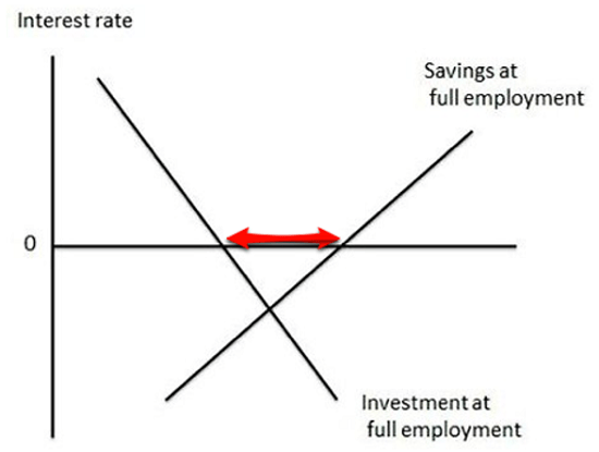
In Wicksell’s model, if the interest rate is too high, S>I and the gap between the two is the amount of hoarding. Unfortunately, this crucial idea is only partially incorporated into Keynesian analysis. Zoltan Jakab & Michael Kumhof argue that the standard loanable funds model doesn’t make sense because it ridiculously implicitly assumes that banks transfer goods from savers to borrowers in a kind of barter system. In a barter system like that, hoarding would be impossible. In reality, banks create money and whenever you have money, it can easily be hoarded which causes recessions.
Fortunately, the hoarding version of the loanable funds model is implicitly incorporated into the liquidity trap models of monetary policy. President Bush’s chief economist, Greg Mankiw understood this when he calculated that the appropriate Federal Funds interest rate that could have largely avoided much of the 2008 recession was below zero. In Mankiw’s graph below, the blue line shows the interest rate that Mankiw thinks would have minimized hoarding and the red line shows the actual interest rate that the Fed maintained.

The problem during the recession of 2008 was that the Fed cannot make the interest rate go below zero. This situation is called a liquidity trap: when the Fed is trapped because it already cut the interest rate to zero and it cannot reduce interest rates more because nominal interest rates don’t go below zero and that causes excessive hoarding. ‘Liquidity’ means the quantity of money in circulation and when the interest rate is zero, the Fed cannot increase liquidity because when it pumps more money into the banking system, the banks just hoard it rather than lending it out. Hoarded money isn’t really part of the money supply.
Disinflation and hoarding.
Most recessions in modern (industrialized) economies have been caused by hoarding which tends to cause inflation (prices) to drop. When people take money out of the economy and hoard it, there is more output per each dollar being spent which implies disinflation or deflation.
11. Y2/(↓M2) → ↑(Y2/M2) → ↓(M2/Y2) = ↓P
Equations 10 and 11 illustrate how hoarding relates to the “quantity theory of money”:
12. MV=PY
V = Velocity of money: a measure of how often each dollar of money is spent on average. I simplified equations 10 and 11 by setting V=1 which means that each dollar was spent once (on average).
Velocity usually doesn’t change much, so we can mostly ignore it.*** Thus when there is an increase in hoarding, that effectively decreases the amount of money (↓M) which must decrease the amount of nominal GDP = ↓(PY). Because prices (P) tend to be sticky, hoarding usually causes real GDP to drop (↓Y) rather than causing a drop in prices (deflation), but sometimes there is some of both.
Footnotes:
*Historical examples of macro models that tried to show general equilibrium include Léon Walras’ Elements of Pure Economics, Arrow-Debreu‘s general equilibrium, and real business cycle theory. John Cassidy explored the tendency of mathematical economists to look for equilibrium in his excellent book including chapters entitled “the mathematics of bliss” and the “perfect markets of Lausanne.” Microeconomic models also tend to assume equilibrium by incorporating ideas like “nonsatiation” which means that people always want to consume more. Nonsatiation is the antithesis of Keynes’ idea of hoarding. Mr Keynes actually wrote a lot more about ‘hoarding’ than ‘saving’ in his 1937 essay The General Theory of Employment, but he never formalized his ideas into equations. In 1937 Keynes wrote that he expected others would collaborate on how to express them into equations:
I am more attached to the comparatively simple fundamental ideas which underlie my theory than to the particular forms in which I have embodied them, and I have no desire that the latter should be crystallized at the present stage of the debate. If the simple basic ideas can become familiar and acceptable, time and experience and the collaboration of a number of minds will discover the best way of expressing them.
Classical macroeconomics had been based on equilibrium models at the time and other economists took Keynes’ stories and tried to translate them into math. The “Keynesian” equations were most notably authored by John Hicks in an essay titled “Mr. Keynes and the Classics” in which Mr. Hicks tried to make sense of Keynes’ ideas using classical frameworks. Classical economics had assumed that S=I so perhaps that is how this pernicious idea entered the standard Keynesian model. Let me know if you find evidence that this is how it happened.
**All economists realize that S=I is actually a simplification that assumes a closed economy with zero net exports (NX). So S=I isn’t really a law even by the standard model which really says:
S-I=NX (Savings-Investment = NetExports)
I left out international trade as a simplification and it isn’t a particularly bad simplification for a large economy like the US because NX usually doesn’t change much as a percent of GDP in large economies.
***Although economists tend to ignore velocity as though it were a constant, official measures of velocity occasionally appear to fluctuate greatly. But velocity is never directly measured so nobody knows how much it really fluctuates. Velocity is calculated using a rearranged equation 12: V=PY/M. We directly measure the other three variables (P,Y,&M), and use them to calculate V. But because we do not directly measure V, it’s calculation is influenced by measurement errors in all the other three variables. One way to explain drops in our calculations of velocity is that they are probably caused by jumps in hoarding which is also unmeasured and when hoarding rises, the effective money supply falls. Our measurements of M cannot account for how much of the money is being hoarded, so we cannot measure when hoarding rises and economists tend to forget that it exists! Rather than infer hoarding, economists infer that a decrease in nominal GDP is due to a drop in velocity which they calculate based on equation 12. It would be more reasonable to assume that it is due to an increase in hoarding because there is no direct evidence that people suddenly become slower to spend money (↓V) during recessions.
 A more intuitive explanation is that hoarding rises during the recessions (shaded columns) which shrinks the remaining effective money supply. An alternative interpretation is that a decrease in velocity (holding on to money longer and spending it more slowly) is just another way of hoarding money.


Leave a Comment